Ending on a High Note — Kaiwalya Kher

I was writing a frequency sweep (a chirp, in DSP terms), a tone that starts at a low pitch and slides up to a high one, like the sound a theremin makes when you move your hand slowly. Mine was supposed to go from 20 Hz (a deep rumble) to 20 kHz (the upper edge of hearing) over three seconds. Simple enough: at each instant in time, figure out what frequency the tone should be at, and play that.

Except it did not work. The pitch climbed at twice the slope it should have, and by the end of the three seconds it had overshot to roughly 40 kHz instead of landing at 20. The first sample was correct. Every sample after that was wrong, and the error grew over time.

The cause turned out to be a piece of math that looks trivial in the constant-frequency case but is sneakily different once the frequency starts moving. The fix is small, but the insight behind it changed how I think about sine waves in general. The punchline: $\sin(2\pi\,\theta(t))$ is a better mental model of a tone than the textbook $\sin(2\pi f t)$ , and here’s why. Along the way I’ll line the problem up next to a car driving down a road, because the exact same mistake on the linear side would be obvious to anyone.

From the Hifi project, a Zig audio experiment. The relevant code is src/processor/sweep.zig in kaiwalya/hifi (pinned to commit 0600cc0, lines 42–49 show the fixed integral).

The analogy, up front

This whole post is really one idea, dressed up in two costumes. On the left is a car moving in a straight line. On the right is a sine wave, which is a point moving around a circle. In both cases there is a rate (speed for the car, $v$ , in m/s; frequency for the wave, $f$ , in Hz) and an accumulation of that rate over time (distance for the car, $d$ , in meters; phase for the wave, $\theta$ ). Both setups share a duration ( $T$ ) and a time variable ( $t$ ).

A quick unit-choice note. I’ll measure phase in cycles (also called turns): one full rotation around the circle equals 1. This keeps the formulas clean. Converting back to the radians that $\sin$ wants is a one-line bookkeeping step at the very end; it doesn’t affect any of the reasoning along the way. Think of it like setting $c = 1$ in relativity to keep the physics readable.

With that, every step of the argument shows up in both columns, because the math is identical.

The setup

Linear motion

A car drives in a straight line. At any instant, it has a speed $v(t)$ in m/s. The odometer reads the total distance $s(t)$ traveled, in meters.

Speed is the rate of change of distance:

v(t) = \frac{ds}{dt}

Equivalently, distance is the accumulation of speed.

Sine wave

A sine wave is a point moving around a unit circle. At any instant, the angle advances at some rate we call the frequency, $f(t)$ , in Hz (cycles per second). The total angle so far is the phase $\theta(t)$ , in cycles.

Frequency is the rate of change of phase:

f(t) = \frac{d\theta}{dt}

Equivalently, phase is the accumulation of frequency.

The easy case: constant rate

Linear motion

A car on cruise control at speed $v$ . After $t$ seconds, the odometer reads:

s(t) = v\,t

Speed times time gives distance. This is the formula everyone internalises before they learn any calculus.

Sine wave

A pure tone at a constant frequency $f$ . After $t$ seconds, the phase has advanced:

\theta(t) = f\,t

Frequency times time gives phase. A 440 Hz tone has accumulated 440 cycles after one second.

The rate starts varying

Linear motion

Now the car is accelerating. Pick the simplest case: linear acceleration from $v_0$ to $v_1$ over duration $T$ :

v(t) = v_0 + (v_1 - v_0)\,\frac{t}{T}

The speedometer needle sweeps from $v_0$ up to $v_1$ over $T$ seconds.

Sine wave

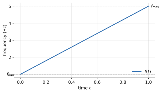
Now the frequency is changing. The Hifi sweep ramps linearly from $f_\text{min}$ (20 Hz) to $f_\text{max}$ (20 kHz) over $T$ (three seconds):

f(t) = f_\text{min} + (f_\text{max} - f_\text{min})\,\frac{t}{T}

The pitch slides from a low hum to a high whine over $T$ seconds.

Linear frequency ramp from f_min to f_max over duration T

The tempting shortcut, which is wrong

Here is where the trap springs. In both worlds, you have a varying rate and you have the constant-case formula fresh in your head. The tempting move is to just substitute: wherever the constant rate appeared, plug in the current value of the varying rate.

Linear motion

“I’m going 60 mph and I’ve been driving for 2 hours, so I’ve gone 120 miles.”

s(t) \stackrel{?}{=} v(t)\,t

If you started at 20 and accelerated up to 60, this is wrong. You did not drive 120 miles; your average speed was lower than 60, so the actual distance is less. Multiplying current speed by elapsed time overstates the distance.

Sine wave

“The constant-tone phase is $f\,t$ ; I’ll just put the varying $f(t)$ in place of $f$ .”

\theta(t) \stackrel{?}{=} f(t)\,t

Same mistake, same reason. The phase $f(t)\,t$ overstates how far around the circle you’ve actually gone. The pitch you hear is not $f(t)$ , and the sweep arrives at a higher frequency than $f_\text{max}$ .

The product rule makes the error explicit

What does the shortcut actually compute? Differentiate its output and see what rate you’d have had to be going to produce that accumulation.

Linear motion

Take the derivative of the wrong $s(t) = v(t)\,t$ to see what “apparent speed” this implies:

\frac{d}{dt}\bigl[v(t)\,t\bigr] = v(t) + t\,v'(t)

That second term is extra. With linear acceleration, $v'(t) = (v_1 - v_0)/T$ , so $t\,v'(t)$ is exactly the ramp portion of $v(t)$ , added a second time. The shortcut acts as if you’d been accelerating twice as aggressively as you actually were.

Sine wave

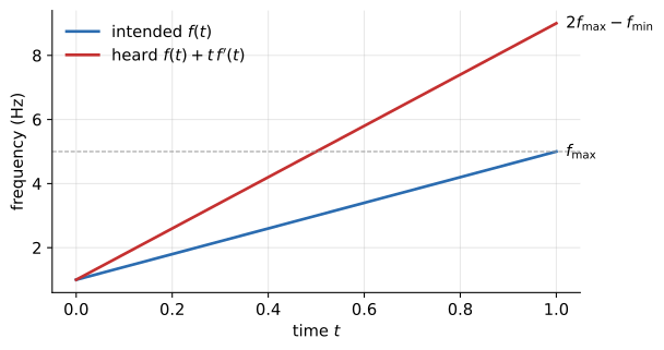
Take the derivative of the wrong phase $\theta(t) = f(t)\,t$ to recover the heard frequency:

f_\text{heard}(t) = f(t) + t\,f'(t)

Same structure. With the linear sweep, $f'(t) = (f_\text{max} - f_\text{min})/T$ , so $t\,f'(t)$ is the ramp portion of $f(t)$ added a second time. The heard pitch ramps at double the intended slope.

The $t\,v'(t)$ and $t\,f'(t)$ terms are the cost of the lie. Intuitively: “current rate times elapsed time” retroactively rewrites history. It treats every earlier moment as if it had happened at the current rate, not the actual (lower) rate it had at the time. The faster the rate is changing, the bigger the lie.

Intended f(t) vs heard f(t) + t·f'(t); the heard ramp has double the slope

The fix: integrate

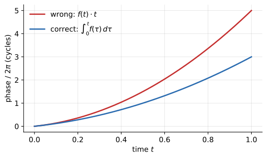
A real odometer does not multiply. It adds up every little bit of distance as it happens. That is an integral, and in code it is a running accumulator (a phase accumulator, on the sine side). When the rate is constant the integral collapses to a multiplication; when the rate varies, you have to actually do the sum.

Linear motion

s(t) = \int_0^t v(\tau)\,d\tau = v_0\,t + (v_1 - v_0)\,\frac{t^2}{2T}

The first term is the “cruise control” distance: what you’d get if the car had held its starting speed $v_0$ the whole time. The second term is the correction for the acceleration, quadratic in $t$ , with the famous $\frac{1}{2}$ factor that shows up in $\frac{1}{2}a t^2$ for uniform acceleration.

Sine wave

\theta(t) = \int_0^t f(\tau)\,d\tau = f_\text{min}\,t + (f_\text{max} - f_\text{min})\,\frac{t^2}{2T}

The first term is the “cruise control” phase: what you’d get from a constant tone at $f_\text{min}$ . The second term is the correction for the sweep, quadratic in $t$ , with the same $\frac{1}{2}$ factor. Not a coincidence: it is the same $\frac{1}{2}$ as the car’s, because the math is literally the same.

Sanity-check either column by differentiating the accumulation and recovering the rate cleanly. The product rule does not bite, because there is no product.

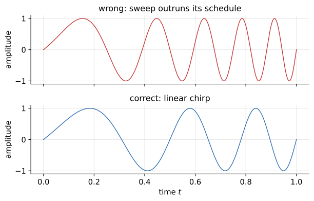
Phase over time: the wrong product f(t)·t diverges above the correct integral

And the waveforms. Same $f_\text{min}$ , $f_\text{max}$ , $T$ , same intention, different reality:

Two waveforms: the wrong version sweeps to a higher pitch than the correct linear chirp

Why this is easy to miss (on the radial side)

On the linear side, nobody makes this mistake. Every physics student learns $d = v_0 t + \frac{1}{2} a t^2$ for uniform acceleration. “Speed times time” for a changing speed is obviously wrong the moment you write it down. The car’s odometer is a concrete object you can point at.

On the radial side, the textbook formula for a pure tone hides the structure. The $f t$ inside is already a disguised integral, just one where the integrand happens to be constant so the integral simplifies to a product. Generalising by swapping $f$ for $f(t)$ preserves the shape of the formula but silently changes the operation from “evaluate a degenerate integral” to “multiply two things.” The step was invisible when the rate was constant. When the rate varies, that hidden step is the whole problem.

The mental model I kept

From this point on I stopped thinking of a sine wave as $\sin(2\pi f t)$ . That form is a trap: it hard-codes a degenerate integral and looks like a multiplication, and when you generalise the thing you thought you were multiplying, you generalise wrong. I replaced it with:

\text{sample}(t) = \sin\bigl(2\pi\,\theta(t)\bigr)

Framed this way, the question “what sample do I emit at time $t$ ?” stops being a math problem about multiplying $f$ and $t$ . It becomes a bookkeeping problem: track the phase. At every moment, the phase advances by whatever the current frequency is. Constant tone, sweep, vibrato: the machinery is the same. You maintain a running $\theta$ and you take its sine. The sweep gotcha cannot occur because $f(t)\cdot t$ never enters the picture. You never multiply a rate by an elapsed time at all.

In code, this is usually a phase accumulator (the same idea that sits at the heart of a numerically controlled oscillator, or NCO): one variable that increments by $f \cdot \Delta t$ each sample, and stays in $[0, 1)$ . Conceptually, it is an odometer for the sine wave.

Side by side, the two versions look almost the same. One line changes:

Wrong: sin(2π f t)

for each sample at time t:
    f = f_min + (f_max - f_min) * (t / duration)
    output = sin(2 * pi * f * t)

It reads fine. Every line is individually correct. The bug is only visible once you ask what f * t means when f has been changing the whole time.

Right: sin(2π θ(t))

phase = 0
for each sample at time t, step dt:
    f = f_min + (f_max - f_min) * (t / duration)
    phase += f * dt
    output = sin(2 * pi * phase)

The quantity f * t has vanished. Phase is a running sum of tiny increments, each taken at whatever the frequency happened to be at that moment.

The Hifi version takes a closed-form shortcut, using the known integral of a linear ramp rather than a per-sample accumulator, but the idea is identical. See src/processor/sweep.zig (pinned to commit 0600cc0). The comment above the formula even spells out the derivation: ng_disp = integrate ng_v.

See the main Hifi post for the surrounding architecture: SIMD vectors, the processor graph, why Zig for audio.